Oliver S. Smart
(c) 2014,2015 SmartSci Limited (c) 2016 Oliver Smart
HOLE release 2.2.005 (07 August 2016)
1. Introduction
HOLE is a program that allows the analysis and visualisation of the pore dimensions of the holes through molecular structures of ion channels Smart et al., 1996. It was written by Oliver Smart while a post doc and independent research fellow at Birkbeck College with the assistance of several students: Guy Coates, Joe Neduvelil, Valeriu Niculae and Xiaonan Wang.
The first application of HOLE was to analyse the pore dimensions of gramicidin A Smart et al., 1993 working with Prof.'s Julia Goodfellow and Bonnie Wallace. For many years HOLE was hosted by Prof Mark Sansom at Oxford. However, because I was busy doing other things HOLE became unavailable about a year ago.
Although it was written over 20 years ago, HOLE remains in demand and its main publications have been cited over 800 times.
2. Licence conditions
Licensed under the Apache License, Version 2.0 (the "License"); you may not use this file except in compliance with the License. You may obtain a copy of the License at
Unless required by applicable law or agreed to in writing, software distributed under the License is distributed on an "AS IS" BASIS, WITHOUT WARRANTIES OR CONDITIONS OF ANY KIND, either express or implied. See the License for the specific language governing permissions and limitations under the License
3. How to setup HOLE from a binary distribution
The HOLE suite is now distributed from its homepage http://www.holeprogram.org and you can get binary distribution from there.
Download the compressed tar ball relevant for your system e.g., hole2.2_003_linux64.tar.gz and place it in your home directory. Unpacking this tar ball will create the directory hole2 containing files for your distribution. Use the commands:
cd
tar xf hole2.2.003.linux64.tar.gz
These commands will create the directories:
-
hole2/doc/index.html is the main documentation (this file).
-
hole2/exe contains the main executables
-
hole2/rad contains a the radius set files needed by hole
-
hole2/examples contains a series of example input files for example runs with hole.
To run the HOLE program and the other executables you can just type the full name of the program. To test that the executable works on your computer by typing at the unix prompt:
~/hole2/exe/hole
*** Program HOLE ***
(edited for brevity)
Control variables read:
The hole program should start and wait for input - hit ctrl-d (the control and d keys together) to get out of this or ctrl-c to interupt. If the program fails to load then please ask for help see http://www.holeprogram.org.
It is normally most convenient to add the hole executable directory to the the unix path (this would allow hole to be started by typing "hole"). Suppose user "mary" has set up the package.
If you are a tcsh or csh user add the following line at the end of your ~/.cshrc file
setenv PATH "$PATH":~mary/hole2/exe
or otherwise if you are a bash user add the line that follows to the file that is used to set your ENV. This file is normally called following ~/.bashrc or ~/.profile or \~/.kshrc
PATH=$PATH:~mary/hole2/exe
|
|
if unsure which shell you are running enter the command echo $SHELL |
Open a new shell (if unsure about this logout and then log back into your terminal). You should be able to run the HOLE executables by typing the command name - try it out by typing hole if there is an error then make sure that you have permission to use the executables by typing ls -l ~mary/hole2/exe. If you cannot see list the directory then go and speak to Mary who should change the permissions for the top hole2 directory (chmod a+rx ~/hole2).
Unless you have installed hole in your own space you will need to modify the examples provided to point to the correct radius files. When specifying a file for vdw radii (using a RADIUS card) you can use files in mary’s area e.g., specify the following line in the
control file: radius ~mary/hole2/rad/simple.rad
|
|
HOLE now resolves ~'s for user names. |
4. Example Application
The best way to show how to run HOLE is to use an actual example. For an example we will use an NMR structural of the gramcidin A channel, determined by Arseniev and co-workers 1GRM. This supplied as an example with HOLE. So the first thing is to copy the files into a convenient convenient directory and then cd into it:
cp -a ~/hole2/examples/01_gramicidin_1grm hole_test
cd hole_test
The ls command should then show that the directory contains the files
1grm_single.pdb hole.inp
4.1. Running HOLE
HOLE is a rather old-style program that by defaults reads from standard input (the keyboard) and writes in text type output to standard output (your terminal window). So to usefully run HOLE you must redirect both input and output to a file. For example:
hole < hole.inp > hole_out.txt
Here the program input is provided by file 01_example.inp and all input goes to file hole_out.txt. The command should complete almost instantly.
|
|
If this is all new to you then Google Command line redirection linux tutorial. There excellent tutorials available, for instance http://ryanstutorials.net/linuxtutorial/piping.php |
Lets look at the input file hole.inp
! example input file run on Arseniev's gramicidin structure
! note everything preceded by a "!" is a comment and will be ignored by HOLE
!
! follow instructions in doc/index.html to run this job
!
! first cards which must be  included for HOLE to work
! note that HOLE input is case insensitive (except file names)
coord 1grm_single.pdb           ! Co-ordinates in pdb format
radius ~/hole2/rad/simple.rad   ! Use simple AMBER vdw radii
                                ! n.b. can use ~ in hole
!
! now optional cards
sphpdb hole_out.sph             ! pdb format output of hole sphere centre info
                                ! (for use in sph_process program)
endrad 5.                       ! This is the pore radius that is taken
                                ! as where channel ends. 5.0 Angstroms is good
                                ! for a narrow channel
-
The coord card must be used to specify the input pdb FILE
-
The radius card must also be specified (it is normal to use simple.rad)
-
The sphpdb card is used to output the sphere centres produced by HOLE to a "pseudo-PDB" file. Each of the "ATOM"s in the file has the pore radius in the B-factor and occupancy columns. The sphpdb file is normally used to produce a dot surface or solid-rendered surface (see below).
|
|
It is possible to directly display the sphpdb file in a molecular graphics program. Load the .sph file as a PDB file. For instance, in PyMOL a crude representation of the HOLE surface can be obtained turning showing the files as spheres and using the command alter hole_out.sph, vdw=b to set the vdw radius to be equal to b (the pore radius). This results in a "dumbbell" - it would be much better to convert HOLE objects to PyMOL CGOs but this needs a bit of coding! |
|
|
For complicated channels with multiple routes through them it is possible to combine a number of HOLE .sph files together. |
4.2. Visualization of the results
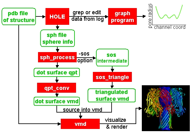
The following diagram summarizes the main methods of visualizing hole results with release 2.2 of hole using the vmd program. There is clear room for improvement and simplification - this will be addressed in future releases.
4.3. Plotting a 2D graph of pore radius vs channel coordinate
One of the more useful ways to visualize the results of HOLE is to plot a graph (all those school teachers/university demonstrators must have some influence). Raw data which can be used for this purpose is written at the end of the run output file. For the gramicidin example text output hole_out.txt is produced. The graph information can be found near the end of the file starting after the line:
cenxyz.cvec radius cen_line_D sum{s/(area point sourc
You can use an editor to extract the information or use egrep:
egrep "mid-|sampled" hole_out.txt > hole_out.tsv
The .tsv file can be opened in most spreadsheets and graphing for instance in excel. On linux I like xmgrace (but it is rather complex) or gnumeric (easier).
gnumeric hole_out.tsv
For the abscissa of the graph it is normal to use the channel coordinate - this is dot product of the sphere centre with the channel vector CVECT. If the channel is aligned along an axis, for instance the y axis (channel vector = {0 1 0}, the channel coordinate will simply be the relevant coordinate. An alternative is to use the distance moved along the pore centre-line from the initial point. The former representation, which was suggested by Mark Sansom, is probably preferable as it allows easy comparison between the results of different runs and for the position of important atoms/residues to be marked on the graph. The latter representation gives an indication of the straightness of the pore but comparison between runs is made more difficult by side to side jumps in the centre line.
It is simple to add some axis labels in gnumeric.
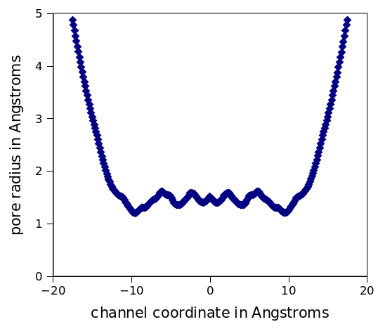
HOLE results on 1grm (spherical probe)
It can be seen that the pore radius within the gramicidin A channel varies between 1.15 and 1.5 Angstroms. Gramicidin A is normally occupied by a single file of around 8 water molecules. For a more detailed coverage see Smart et al., 1993
4.4. Producing a colored dot surface and visualizing in vmd
Being able to visualize HOLE results together with the ion channel model in a molecular graphics program is really useful. HOLE was originally written to work with the Quanta program (in fact a predecessor of Quanta called Hydra). It has conversion tools for a variety of other programs. HOLE really works well with vmd http://www.ks.uiuc.edu/Research/vmd/ and we will look at how to display HOLE graphical objects in vmd.
The starting point for visualizing HOLE results is to produce a surface from the raw HOLE sphere files stored in the .sph file produced by sphpdb option of HOLE. In this example the file is called hole_out.sph.
The simplest surface to look at is a dot surface. To produce a dot surface from hole_out.sph use the sph_process program (supplied with HOLE):
sph_process -dotden 15 -color hole_out.sph dotsurface.qpt
-
The -dotden option is used to increase the number of dots on the surface.
-
The -color option is used to produce a colored surface. Red is where the pore radius is to tight for a water molecule. Green where there is room for a single water. Blue is where the radius is double the minimum for a single.
-
To see more detail and other options run sph_process -h
-
The dotsurface.qpt file code be displayed in Quanta but you probably want to use vmd. So it is necessary to use qpt_conv (at present). This is an interactive program (it seemed like a good idea many years ago). You have to select option D and hit the Enter key three times to do the conversion:
qpt_conv
initial splash message not shown here
This program converts a .qpt file (as produced by hole)
 to something else.
Output options
'A' to/from ascii version of original .qpt (can then edit)
'C' A .qpt file in which dots are replaced by 3D crosses
'L' A .qpt file with long lines split into smaller sections
      (useful for proper depth queueing in qplot)
'I' InsightII format
'R' Rasmol format
'S' Sybyl format
'K' to David C. Richardson's kinemage format
'O' for use with O program
'V' to Virtual Reality Markup Language
'D' to VMD format
Enter conversion option character <stop program>: D
S/r qptvmd. Reads in a hydra/quanta 3D binary plot and writes out an VMD equivalent. To use this file in VMD type: source blah.vmd_plot at the vmd prompt Please enter input binary hydra/quanta plot (old) filename defaults <dotsurface.qpt> ext:<.qpt> (abort by EXIT or ^D) : Please enter vmd format file (new) filename defaults <dotsurface.vmd_plot> ext:<.vmd_plot> (abort by EXIT or ^D) : What width do you want lines to appear:
-
The end result of this is a file dotsurface.vmd_plot To use this in vmd
-
Start vmd and load 1grm_single.pdb
-
select a pretty graphical representation (here liquorice with tube colored by chain).
-
Then go to the terminal window where you started vmd. Hit the Enter key. You will then see the vmd command prompt:
vmd >
-
At the prompt enter the command:w :
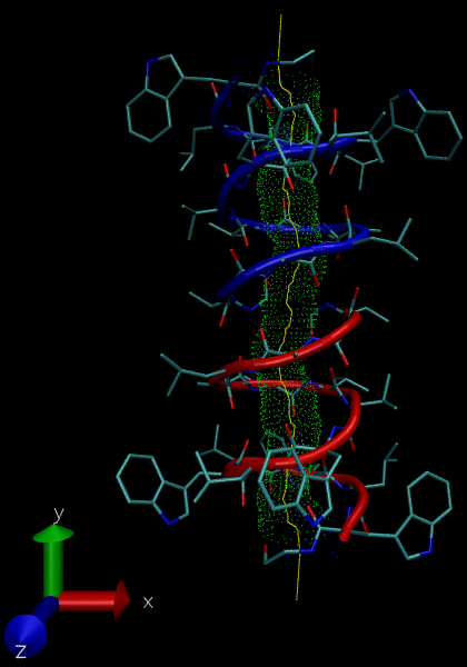
source dotsurface.vmd_plot -
you will then see the dot surface in the VMD window. A great way to make pictures of this is with vmd supplied Tachyon to produce a ray traced result
-
4.5. Producing a triangulated surface and visualizing in vmd
The dot surface is nice (it made me happy in 1993) and is still the most useful way to actually visualize results. However, if you want a pretty picture for poster/paper a solid surface is better.
Producing a triangulated surface is similar to the dot surface. We use hole_out.sph as the starting point and run
sph_process -sos -dotden 15 -color hole_out.sph solid_surface.sos
The .sos is an intermediate file that needs to be processed by sos_triangle
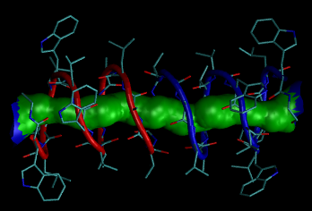
sos_triangle -s < solid_surface.sos > solid_surface.vmd_plot
To load in vmd source solid_surface.vmd_plot at the vmd > prompt (see above). The result is a nice solid surface:
5. Further information
For further information about control cards, please see the old documentation old/index.html for now.
6. Acknowledgements
The support of the UK Science and Engineering Research Council under project grant GR/G49494 and from the Molecular Recognition and Computational Science Initiatives is gratefully acknowledged. I should like to thank Julia Goodfellow and Bonnie Wallace for support and many discussions. Thanks are also due to Mark Sansom and his group at the University of Oxford, and Karen Duca of Brandeis University for testing the first release. In addition thanks to Rod Hubbard and Polygen/Molecular Simulations Inc. for providing the 3D plot file facility in HYDRA and QUANTA. QUANTA is available from Molecular Simulations Inc., Waltham, MA 02154, USA. InsightII is available from Biosym Technologies, 9685 Scranton Road, San Diego, CA 92121 - 2777 USA.
The generous support of the Wellcome Trust by the provision of a Career Development Fellowship for the author is gratefully acknowledged. Much of the work undertaken was encouraged by Dr Mark Sansom and members of his group at the University of Oxford. Thanks to Guy Coates, Joe Neduvelil, Valeriu Niculae and Xiaonan Wang for contributing to the programming as students at Birkbeck.
Thanks to Global Phasing Ltd for the provision of CentOS5 and OSX hosts for building and testing. Thanks to all the initial testers in particular Oliver Clarke.